Build your own Wordle application in Excel without a single line of code.
Which word or phrase was most searched for on Google in 2022? You might guess “World Cup”, “Queen Elizabeth” or “Ukraine”. Indeed, all of these were in the top 10, but the most entered search word in Google in 2022 was… “Wordle”!
For those of you who do not know what Wordle is (where have you been?), it is a very simple word game where one must guess the 5-letter word of the day in 6 guesses or less. With each guess, useful information for future guesses is obtained, based on whether or not any letters were guessed correctly and whether they are in the correct position.
For example, if the Wordle of the Day is CRAZY and you guess TRACK, your guess will be displayed as follows

This means that in the Wordle there is an R and an A in positions 2 and 3 respectively. The C on the other hand is present in the Wordle but is not in the correct position.
And how did Wordle become the most searched for word on Google? Well, it is mostly due to frustrated players looking up the answer to today’s puzzle (cheating in Wordle is rife!)
So, if after this introduction you still haven’t tried Wordle, please do so now as the rest of this article will make much more sense.
Why is Taleo allowing me to write an article about Wordle? Well, they told me to write about something I am an expert in, so it came down to an article about Wordle or a recipe for scones! But they did insist that it should relate in some way to my work as a Business Analyst…
So I am going to show you how to write a simple Wordle application in Excel with zero coding required.
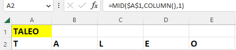
Let’s start by placing the WORDLE in cell A1. Then in cells a2:e2, I place the formula =MID($A$1,COLUMN(),1)
This is to split the 5-letter word into 5 consecutive cells. Note that when I refer to cell A1, I use the $A$1 absolute notation. This is so that when I copy the formula to the right, the cell reference does not change to B1, C1 etc. The COLUMN() function returns the number of the current column (a=1, b=2 etc.) Hence in cell C2, I am taking MID (”TALEO”,3,1) i.e. the third letter of TALEO[1].
Now we need to create a zone to allow the player to input their guesses and display the results.
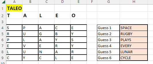
To do this, I have allocated the zone H4:H9, where the player can enter their guesses, and A4:E9 where the results will be displayed. I could have had the player enter the guess directly in the cells A4:E9, but it would have been a little awkward for the user who would have to move between cells with each letter. We are going to use roughly the same formula as before, to split up the guesses across the columns. The formula below is to be entered in A4 and then copied to the grid A4:E9.
=MID($H4,COLUMN(),1)
Note that in the reference $H4 we anchor the reference to column H with the dollar sign, but do not anchor the row reference, allowing it to change as the formulae are copied down.
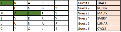
Once this is done, you can test your progress by keying in 6 5-letter words into the cells H4:H9. You should see something resembling the screen below.
Now for the magic!
We are going to use Conditional Formatting to apply the appropriate colours to your guesses. Let’s start with the formatting to show cells where the correct letter has been guessed in the correct position.
First, select the zone A4:E9 where we wish to apply the conditional formatting.
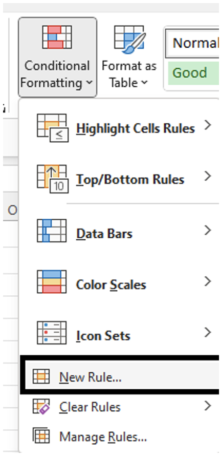
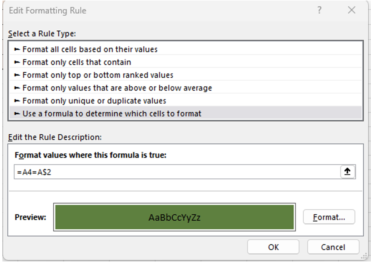
Next, click on the Conditional Formatting button from the Home menu bar and select New Rule. Then choose “Use a formula…” and enter the formula =A4=A$2
Finally do not forget to choose a fill colour using the Format button! (If you do not do this, you will not see any change!)
This formula =A4=A$2 is to identify and format the letters that are present in the Wordle in the correct position.
 |  |
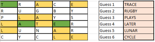
After applying this rule, you should see something similar to the image below (depending on the words you have chosen and the format colour.)
Now we would like to create the rule to detect a correct letter in the wrong position. Again, go to Conditional Formatting to create a new rule using a formula (alternatively you can duplicate and edit the existing rule.) This time enter the following formula.
=HLOOKUP(A4,$A$2:$E$2,1,FALSE)=A4
This formula uses HLOOKUP, the unfairly neglected cousin of VLOOKUP. It looks up the value of the cell horizontally instead of vertically, in the zone $A$2:$E$2 (anchored).
Do not forget to apply a different fill colour than the previous one.
If you are not seeing a result like the one shown above, check that your two rules have been correctly recorded. (Excel does some strange things that I don’t claim to understand.)
If you go into Conditional Formatting / Manage Rules, it should look as below: (note “Show formatting rules for This Worksheet”).
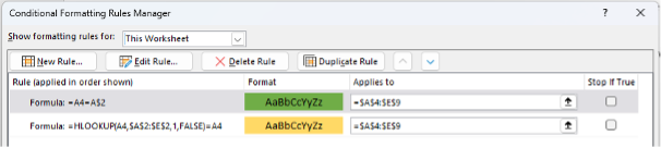
The order of the rules is important to decide which rule takes precedence over another. If necessary, you can move a rule up or down, by selecting it and using the arrows (next to the Duplicate Rule button.)
Obviously, there are a few next steps before you can enjoy all the fun of the original game. Firstly, the WORDLE that you are trying to find should not be visible, otherwise, it is just a little too easy, so one next step is to hide the row containing the word.
And the next step is to randomize the WORDLE so that you are not trying to guess the same word each day.
If there is sufficient interest in a follow-up article, I will show you how to have a different word each day, and other enhancements for the complete Wordle experience – all without a single line of code!
David McKinney, Senior Business Analyst at Taleo Consulting.
[1] I was hoping to use an array function like TEXTSPLIT to split out the WORDLE, but it only works for delimited text (and not fixed width.)